
Online evaluation and A/B testing
Why your offline eval lied about a 3-point lift, the implicit signals that don't, and the sample sizes LLM A/B tests actually need.
A team runs a prompt change against their 100-example eval suite. The new prompt scores 3 points higher than the old one. They ship it. A week later, production metrics are flat. Two weeks later, support tickets are slightly up.
Nothing went wrong with the model. The eval lied. At 100 examples, the smallest accuracy difference you can detect at 80% statistical power is around 10 to 12 points, not 3.[1] The 3-point gain was noise inside the confidence interval, and shipping on it was a coin flip dressed up as a measurement.
Offline evals catch obvious regressions, and Regression suites and CI gates is the chapter for that. But the call on whether a change actually helps users has to come from production traffic. This chapter is about the two things production gives you that a static eval set can't: implicit signals generated by every real user without lifting a finger, and A/B tests that attribute metric movements causally to your change. Both are noisier than they look. The whole game is sample size.
What users do is more honest than what they say#
Thumbs widgets are the most popular eval tool in AI products and one of the worst. Two users press thumbs-down on the same Copilot suggestion: one because the variable name was wrong, one because the entire suggestion was irrelevant. Both produce the same single-bit signal. A third user regenerated the response four times and gave up. They generated no signal at all.
The fix isn't a five-star rating widget. It's measuring what users do with the response, which is generated for free on every interaction. Three tiers, ordered by how confidently each one indicates quality:
Tier 1 is acceptance. Did the user copy the output without editing it? Did they accept the code suggestion verbatim? Did they actually do the thing they came to do (commit the code, publish the document, resolve the ticket)? These are the strongest signals because they're zero-effort: the user kept your output as the final answer. Useful AI writing and code tools see copy-without-edit rates of 25 to 40%; rates below 15% mean the model is producing wrong-shape outputs (as of April 2026).[2] GitHub Copilot tracks suggestion acceptance rate as its primary metric; a Zoominfo deployment study reported 33% suggestion acceptance and 20% line-of-code acceptance across professional developers (as of January 2025).[3]
Tier 2 is diagnostic. Regeneration rate, edit-distance distribution, latency abandonment. These tell you a class of requests is failing, and often how it's failing. Word-level edits mean you got the content right and the tone wrong. Complete deletion-and-rewrite means task-distribution mismatch. The catch is segmentation: technical queries run a 50 to 60% regeneration rate while general queries run 10 to 15%.[2:1] An unsegmented average of those two populations diagnoses neither, and worse, a shift in your traffic mix can flip the aggregate signal without any change in model quality.
Tier 3 is engagement. Does the user come back within 7 days? How deep do conversation sessions go? These are leading indicators of retention. They're noisy at the per-request level but stable in aggregate, and 7-day return is consistently the strongest predictor of 3-month retention across productivity software.[2:2]
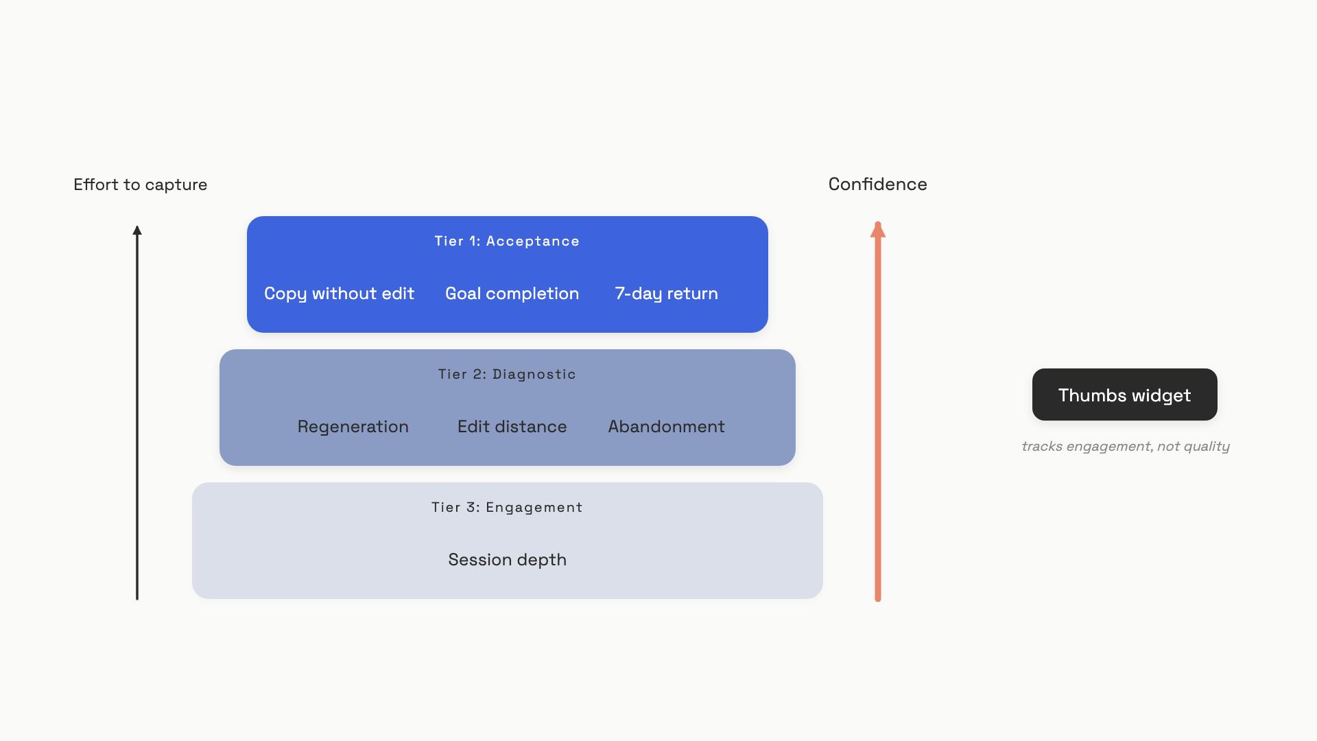 The three tiers of implicit signal, ordered by how strongly each one tracks actual quality. Explicit thumbs ratings sit off to the side because they correlate more with engagement than with quality.
The default for production monitoring is implicit signals at all three tiers, segmented by intent cluster. Use explicit thumbs feedback as a trigger for investigation, not as a primary metric: a thumbs-down means "look at this trace." A study cited by GrowthBook (June 2026) found that thumbs feedback correlates more with overall engagement than with quality.[4] If your dashboard ranks features by thumbs-up rate, you're ranking them by how much users like the product overall, which is the wrong question.
Sampling production traffic#
Implicit signals scale to 100% of traffic for free. Anything deeper than implicit signals (running an LLM-as-judge over the full output, sending traces to a human reviewer, computing semantic similarity against a reference) costs real money per request, and you can't afford to do it on every call. The fix is sampling. Three strategies, each answering a different question.
Random sampling at 1 to 5% of traffic gives an unbiased estimate of population-level quality. It's the right default for a quality dashboard. The risk is that rare-but-severe failure modes (the 0.1% of queries that produce a hallucinated medical dosage) get sampled proportionally to their frequency, which is roughly never.
Stratified sampling fixes that. Cluster requests by intent (semantic embedding of the query is the usual trick), then sample at higher rates from clusters with higher historical error rates or higher business stakes. You're spending the same total review budget but concentrating it where the failures live.
Targeted sampling on low confidence uses a cheap signal to decide which requests get the expensive review. A judge model's uncertainty estimate, ensemble disagreement between two models, or the regeneration signal itself can flag the requests most likely to be failures. This is where LLM-as-judge does double duty: the same judge that scores eval sets can run on a sliver of production traffic, and the requests it scores low get escalated to a human reviewer.
import hashlib
import random

def should_sample(request_id: str, base_rate: float,
                  intent_cluster: str, judge_score: float | None) -> bool:
    """Return True if this request should be deeply evaluated."""
    # Tier 1: deterministic random sample (request_id hashed for stability)
    h = int(hashlib.sha256(request_id.encode()).hexdigest(), 16) / 2**256
    if h < base_rate:
        return True

    # Tier 2: oversample high-stakes intent clusters
    oversample = {"medical": 0.20, "legal": 0.10, "billing": 0.05}
    if h < oversample.get(intent_cluster, 0):
        return True

    # Tier 3: targeted on low judge confidence
    if judge_score is not None and judge_score < 0.4:
        return random.random() < 0.5
    return False
Hashing the request_id instead of rolling a fresh random number means the same request makes the same sampling decision on a replay. That matters when you're debugging an evaluation pipeline and need deterministic behavior.
One more strategy is worth its own name: shadow mode. Before any model or prompt change that's hard to roll back (a fine-tuned model swap, a major prompt rewrite), route real production requests to both the current and the candidate, return only the current to the user, and compare the candidate's outputs offline. Shadow mode gives you real production distribution at zero user risk. The cost is roughly double the inference spend for the duration. Run it for a day or two on 5 to 20% of traffic before exposing the candidate to users.
A warning, because Intercom learned this one expensively: shadow-mode comparisons use offline metrics (semantic similarity, judge scores), and a better offline score does not always mean better business outcomes. Pedro Tabacof at Intercom documented a case where a prompt variant with a lower offline eval score produced better A/B test business results.[4:1] Shadow mode catches obvious distribution failures. The ship-or-not-ship call still belongs to the live A/B test.
Why LLM A/B tests need bigger N#
Classical A/B testing assumes two things that hold for a button-color change and break for an LLM change:[5]
- Per-user variance is small relative to the effect you're trying to detect.
- Each measurement is roughly an independent draw from a stable user-behavior distribution.
LLM features blow up both. Inter-user variance is higher because the input is natural language: two users asking "the same" question phrase it differently, which sends the model into different parts of its output distribution and produces answers with different latencies, lengths, and downstream behaviors. Intra-user variance is high in a way deterministic features have no analog to: the same user asking the same question across two sessions can get materially different answers due to temperature, retrieval freshness, and floating-point non-determinism in parallel GPU execution. One study documented statistically significant performance differences (p=0.013) between identical model weights running on two cloud providers.[5:1]
The practical consequence: an LLM feature has 2 to 5 times the variance of a deterministic feature.[5:2] A standard sample-size calculator fed historical variance numbers from your last button experiment returns a number that's wrong by that same factor. You need 2 to 5 times the sample size, or 2 to 5 times the experiment duration, to reach the same statistical power.
The number every team should run before starting an experiment:
import math
from scipy.stats import norm

def ab_sample_size(p_baseline: float, p_treatment: float,
                   alpha: float = 0.05, power: float = 0.80) -> int:
    """Required N per arm for a two-proportion z-test."""
    z_alpha = norm.ppf(1 - alpha / 2)
    z_beta = norm.ppf(power)
    var1 = p_baseline * (1 - p_baseline)
    var2 = p_treatment * (1 - p_treatment)
    delta = abs(p_treatment - p_baseline)
    return math.ceil(((z_alpha + z_beta) ** 2 * (var1 + var2)) / (delta ** 2))

for lift in [0.10, 0.05, 0.03, 0.02]:
    print(f"Lift={lift:.0%}: N per arm = {ab_sample_size(0.82, 0.82 + lift)}")
Run it from a baseline of 82% and the output is sobering:
| Effect you want to detect | N per arm |
|---|---|
| 10 percentage points | 210 |
| 5 percentage points | 870 |
| 3 percentage points | 2,400 |
| 2 percentage points | 5,400 |
To reliably detect a 3-point lift at 5% significance and 80% power, you need roughly 2,400 examples per arm.[1:1] The average internal eval suite has 50 to 200 hand-curated examples. At 100 examples, the smallest lift you can detect is 10 to 12 points, not 3. Anything below that is the test telling you it doesn't know.
The relationship is quadratic: standard error shrinks with the square root of N, so halving the effect size you want to detect quadruples the sample size you need.
LLM stochasticity makes this worse. Run the same model twice on the same eval set and the score moves. Lumiste's 2023 demonstration on a 64-case set showed GPT-4 accuracy bouncing between 65% and 75% across consecutive identical runs.[6] If the variation from running the test twice is 10 points, a 73% baseline versus a 76% treatment isn't a result; it's a coin flip you got to call twice.
Stopping an A/B test early when p drops below 0.05 inflates your false positive rate. Checking the dashboard 20 times during a fixed-horizon experiment with nominal alpha=5% pushes the true false positive rate to roughly 40%.[7] If you need to peek, use sequential testing (alpha-spending or always-valid inference); if you don't, set N in advance and run to completion. Pre-register the stopping rule before the experiment starts.
The single most useful variance-reduction technique for LLM A/B tests is paired analysis. When both arms evaluate identical questions or identical users, compute the per-question or per-user difference instead of comparing means across pooled groups. The covariance between arms (driven by question difficulty or user heterogeneity) cancels out, and the residual variance is what your treatment actually moved. Anthropic's statistical evals work documented frontier-model question-score correlations between 0.3 and 0.7 on popular benchmarks; paired analysis on a correlation of 0.5 cuts required N roughly in half.[8] A paired version of the 3-point detection scenario drops from 2,400 per arm to about 1,200.
For experiments with established users, CUPED (Controlled-experiment Using Pre-Experiment Data) is worth knowing about: you regress out the predictable component of each user's outcome using their pre-experiment behavior on the same metric, and the residual variance shrinks by a factor of 1 minus the squared correlation. With a correlation of 0.7 between pre- and post-experiment behavior (typical for engagement metrics), CUPED reduces variance by about 51%, equivalent to running 2x the sample size at no extra cost.[9] CUPED stops helping when most of your users are new (no pre-experiment data) or when the treatment changes the feature so substantially that pre-experiment behavior no longer predicts post-experiment behavior.
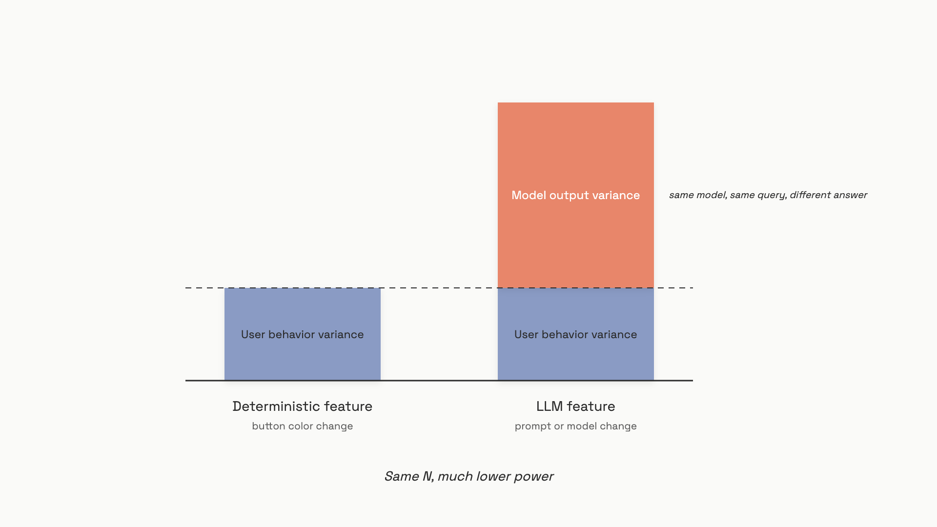 A deterministic feature has one source of variance; an LLM feature stacks model-output variance on top, which is why the same N produces a much weaker test.
The pipeline that ties it together#
The discipline that emerges from all of this is a three-stage funnel, not a single decision point. Offline evals filter the obvious failures. Shadow mode surfaces production-distribution issues the offline set didn't anticipate. Live A/B with adequate N makes the ship-or-not-ship call against business metrics. Each stage catches a different class of problem, and skipping any of them either ships a regression or wastes traffic on changes a 30-line eval would have killed for free.
The Intercom case is the clearest illustration: a prompt with the worse offline score won the A/B test, and the team's takeaway was that they "rely much less on intermediate evals now, and let production data make the call."[4:2] That doesn't mean offline evals are worthless; it means offline evals are a filter, not a verdict. Use them to kill obvious losers cheaply. Use the A/B test to pick the winner.
The number to remember when you're scoping the A/B is 2,400 per arm for a 3-point lift at 80% power. If your traffic doesn't support that within a reasonable experiment window, you have three honest options: target a larger effect size (and accept that small wins will be invisible), apply paired analysis or CUPED to cut the required N, or report the offline result with explicit confidence intervals and stop pretending the eval can answer a question it doesn't have the resolution to answer. The trap is the fourth option, which is shipping on the underpowered result and discovering in production what you should have admitted in the calculator.
Implicit signals are the layer that lets you keep evaluating after the experiment ends. Once a change is live, copy-without-edit rate, segmented regeneration rate, and 7-day return are how you notice that the win held, the win faded, or the win was an artifact of novelty in the first cohort. They cost nothing extra, they cover 100% of traffic, and they're harder to fool than any rating widget. The work is in instrumenting them once and segmenting them carefully forever.
At architecture scale, Observability for AI Systems covers the whiteboard view of metrics pipelines and experimentation infrastructure. The next chapter, Tracing, is what makes the request_id-keyed event stream this chapter assumes you have.
References#
Tian Pan, "Your LLM Eval Is Lying to You: The Statistical Power Problem," April 15, 2026. https://tianpan.co/blog/2026-04-15-llm-eval-statistical-power ↩︎ ↩︎
Tian Pan, "Behavioral Signals That Actually Measure User Satisfaction in AI Products," April 20, 2026. https://tianpan.co/blog/2026-04-20-behavioral-signals-ai-products ↩︎ ↩︎ ↩︎
arXiv 2501.13282, "Experience with GitHub Copilot for Developer Productivity at Zoominfo," January 2025. https://arxiv.org/abs/2501.13282 ↩︎
GrowthBook, "How to A/B Test AI Features," June 10, 2026. https://blog.growthbook.io/how-to-a-b-test-ai-a-practical-guide/ ↩︎ ↩︎ ↩︎
Tian Pan, "Variance Eats the Experiment: Why A/B Power Math Breaks for LLM Features," April 27, 2026. https://tianpan.co/blog/2026-04-27-ab-test-power-stochastic-features ↩︎ ↩︎ ↩︎
Martin Lumiste, "Why You Should A/B Test Your LLM Evals," August 2023. https://mlumiste.com/technical/ab-test-llm-evals/ ↩︎
Statsig, "Sequential Testing: How to Peek at A/B Test Results Without Ruining Validity," June 23, 2025. https://statsig.com/perspectives/sequential-testing-ab-peek ↩︎
Anthropic, "A Statistical Approach to Model Evaluations," November 19, 2024. https://www.anthropic.com/research/statistical-approach-to-model-evals ↩︎
Statsig, "CUPED Explained," September 15, 2024. https://www.statsig.com/blog/cuped ↩︎