
Embeddings and vector search
How to pick an embedding model on your own data, why pgvector is the default store, what HNSW and IVFFlat actually do, and the honest threshold where a dedicated vector DB earns its keep.
You already know what an embedding is. This chapter is about the four decisions that come next, in the order most teams hit them: which model to embed with, where to put the vectors, what kind of index to build over them, and when to stop using PostgreSQL and pay for something specialized.
Three of those four decisions have a strong default. The fourth, model selection, is the one teams reliably get wrong because the evidence they reach for, MTEB rank, doesn't measure what they need it to. So we'll start there.
Don't pick your embedding model from a leaderboard#
The Massive Text Embedding Benchmark (MTEB) ranks embedding models on 56 public tasks: Wikipedia retrieval, news classification, legal text similarity, and a few dozen cousins.[1] As of early 2026, Google's Gemini Embedding 001 leads the English board, Alibaba's Qwen3-Embedding-8B leads multilingual, and Voyage-3-large is the strongest hosted-API option.[1:1]
None of those rankings tell you how a model performs on your Salesforce opportunity notes, your pharmaceutical trial summaries, or your internal engineering tickets. MTEB averages across public corpora; a model ranked eighth overall can beat the top-ranked model on your domain if its pretraining distribution happens to match your text better.[1:2] There's also a contamination tail: several top-ranked MTEB models have been documented training with partial access to benchmark test sets, so even the public ranking is partly inflated.[2]
The fix is the same discipline your first eval set preached for prompts, applied to retrieval:
- Pull 500 to 2,000 representative documents from your actual corpus.
- Write or harvest 100 to 200 real user queries with known relevant documents. (An afternoon's work; the set is reusable for every future model comparison.)
- Embed both with each candidate model, run nearest-neighbor search, compute Recall@5 and MRR@10.
- Pick the cheaper model if the gap is under five points. Pick the better one if it's not.
That's the entire process. It beats reading leaderboards every time, and once you have the eval set, you also have the early-warning system for the day a hosted provider silently swaps model weights underneath you.
A reasonable starting shortlist for that eval, in mid-2026:
text-embedding-3-smallat 512 dims ($0.02 per million tokens as of June 2026[3]). Cheap, supports Matryoshka truncation, the right default for most teams to test first.text-embedding-3-large($0.13 per million tokens[4]) when small loses by more than five Recall@5 points, or when the corpus is multilingual (large beats ada-002 by 23 points on MIRACL[4:1]).voyage-3-large($0.18 per million tokens[5]) for code-heavy or specialized English corpora where it's known to do well.bge-m3orarctic-embed-2.0self-hosted when monthly volume crosses ~500M tokens and the API math flips, or when vendor model-version risk is contractually unacceptable.
The dimensions knob is worth using. Both text-embedding-3-* families and several open-source models are trained with Matryoshka Representation Learning, which means you can ask the API for 256 or 512 dims and get a usable lower-quality vector instead of the default 1,536 or 3,072.[6] OpenAI's own data shows text-embedding-3-large truncated to 256 dims still beating full-size ada-002 at 1,536 on MTEB.[4:2] That's a two-thirds storage cut and a noticeably faster index, for free.
# OpenAI: ask for shorter vectors at embedding time
from openai import OpenAI
client = OpenAI()

resp = client.embeddings.create(
    model="text-embedding-3-small",
    input=["the cat sat on the mat"],
    dimensions=512,  # Matryoshka truncation; default would be 1536
)
vec = resp.data[0].embedding  # length 512
Run your eval at the truncated dimension before assuming you need the full one. Most corpora don't notice.
pgvector is the default store#
For new RAG workloads, the right vector store is a PostgreSQL table with the pgvector extension installed. Not Pinecone, not Qdrant, not Weaviate. PostgreSQL.
The argument is operational, not ideological. You almost certainly already run a Postgres instance. CREATE EXTENSION vector adds a vector(N) column type and four similarity operators (<=> for cosine, <-> for L2, <#> for inner product, <+> for L1) that plug into normal SQL.[7] Document text, metadata, embeddings, and tenant IDs all live in the same row. WHERE tenant_id = $1 filtering works on day one without a separate "payload index" feature. Your existing backups, replication, and observability cover the vector store for free. There's no second database to deploy, monitor, version, or pay AWS egress to talk to.
Setup is four lines:
CREATE EXTENSION IF NOT EXISTS vector;

CREATE TABLE documents (
    id        bigserial PRIMARY KEY,
    tenant_id text NOT NULL,
    content   text NOT NULL,
    embedding vector(512)
);

CREATE INDEX ON documents
    USING hnsw (embedding vector_cosine_ops)
    WITH (m = 16, ef_construction = 64);
Querying is a normal SELECT with an ORDER BY on the distance operator:
SELECT id, content, embedding <=> $1 AS distance
FROM documents
WHERE tenant_id = $2
ORDER BY distance
LIMIT 10;
That's the whole interface. No SDK, no auth tokens, no separate retry policy.
The "pgvector is a toy" reflex is several years out of date. In May 2025 Timescale ran the open ann-benchmarks suite at 50 million 768-dim Cohere embeddings on a single AWS r6id.4xlarge ($835/month on-demand, 128 GB RAM). pgvector with the pgvectorscale extension hit 471 queries per second at 99% recall; Qdrant on the same hardware hit 41 QPS at the same recall.[8] Postgres won throughput by 11x. Qdrant won p99 tail latency (39 ms vs 75 ms at 99% recall) and built the index in a third of the time. Both numbers are real. Neither says "you must migrate."
What pgvector cannot do gracefully:
- Native horizontal sharding. Postgres scales by getting a bigger box, not by adding nodes. Read replicas help reads; they don't shard the index.
- Index 3,072-dimension vectors directly. The
vectortype's HNSW and IVFFlat indexes are capped at 2,000 dimensions. Fortext-embedding-3-largeat full size, you either truncate at embedding time, store ashalfvec(3072)(FP16, indexed up to 4,000 dims), or binary-quantize to abitcolumn.[9] - Build very large indexes fast. The 50M index above took 11 hours to build on pgvectorscale's StreamingDiskANN, versus 3.3 hours on Qdrant.[8:1] If you reindex weekly, that gap matters.
None of those are deal-breakers under 10 million vectors. We'll come back to the threshold.
HNSW and IVFFlat in plain terms#
Sequential scan over a million vectors is slow. The AWS pgvector benchmark on 58,000 1,536-dim vectors clocked sequential scan at 650 ms per query; with an HNSW index, the same query took 1.5 ms.[10] That 400x gap is what an approximate-nearest-neighbor (ANN) index buys you, in exchange for a sliver of recall.
pgvector ships two ANN indexes. They work very differently, and the choice between them is one of the few decisions in RAG with a real consensus answer.
HNSW (Hierarchical Navigable Small World) builds a multi-layer graph. Every vector becomes a node. Each node has edges to its nearest neighbors, with a few long-range edges sprinkled at the top layers and dense local connections at the bottom. To find the nearest neighbor of a query, you start at the top layer, walk greedily toward whichever neighbor is closest to the query, drop down a layer when you can't get any closer, and repeat. The top layers fly you across the space; the bottom layer pinpoints the answer.
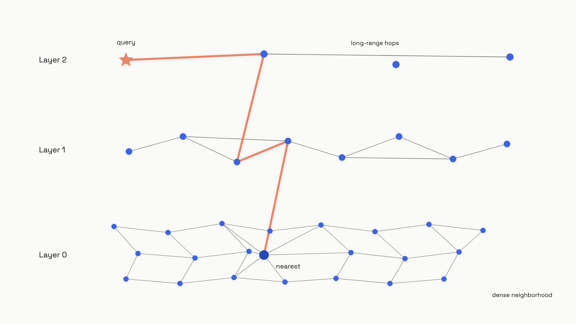 HNSW navigates from sparse top layers to the dense bottom in a few hops. The query never visits most of the graph.
Three knobs, all with sensible defaults:
m(default 16): edges per node. Higher means denser graph, better recall, more memory. Production range is 12 to 48.ef_construction(default 64): how hard the builder works to find good neighbors when inserting. Must be at least2*m.hnsw.ef_search(default 40): how hard the query works at lookup time. Set withSET hnsw.ef_search = 100;per session. Raise it if recall is below your target.
HNSW has two properties that matter for production. First, you can build the index on an empty table and it absorbs inserts cleanly forever after. Second, the recall-vs-latency curve is excellent at the defaults: 95%+ recall out of the box on most workloads.[11]
IVFFlat is the older, simpler design. At build time it runs k-means over the existing vectors and partitions the space into lists Voronoi cells, each anchored on a centroid. At query time it computes the distance from the query to every centroid, picks the probes nearest cells, and scans only the vectors inside those cells.
Two knobs:
lists: number of cells. pgvector recommendsrows/1000up to a million rows, andsqrt(rows)past that.[11:1]ivfflat.probes(default 1): how many cells to scan at query time. Recommended starting value islists/10(orsqrt(lists)past a million).
IVFFlat has one trap that has bitten more teams than any other pgvector pitfall. The index must be built after the table has representative data. If you create an IVFFlat index at schema-creation time (which most ORMs and migration tools do by default), k-means runs on near-zero rows, every centroid lands in roughly the same place, and queries return garbage with no error.[12] Supabase's docs put it bluntly: "Building an IVFFlat index on an empty collection will result in significantly reduced recall."[12:1]
Side by side:
| HNSW | IVFFlat | |
|---|---|---|
| Build on empty table | Yes | No, breaks silently |
| Memory | 2 to 5x more | Less |
| Build time | Slower | Faster |
| Query latency at 95% recall | Lower | Higher |
| Handles inserts | Yes, no rebuild | Drifts; rebuild advised |
| Recall over time | Stable | Degrades as data shifts |
The decision rule is short: default to HNSW for everything new. Use IVFFlat only when the dataset is essentially static, you're memory-constrained, and faster initial build time matters more than steady-state query speed. There's no live debate on this in the literature; HNSW won the trade-off comparison for online workloads several years ago and the gap hasn't closed.
One additional 0.8.0 feature worth knowing: HNSW now supports iterative scans (SET hnsw.iterative_scan = ON), which keeps walking the graph until enough results pass your WHERE filter.[13] Before that, a high-selectivity filter on a multi-tenant table could starve the result list and quietly tank recall. If you're on multi-tenant pgvector, turn it on.
When you actually need a dedicated vector DB#
Most teams pick Pinecone or Qdrant in week one, before they have any measured reason to. The cost is real and recurring: another piece of infrastructure with its own API keys, network egress bill, backup procedure, monitoring story, and on-call rotation. The benefit is conditional on workloads they don't have yet.
The honest threshold map, based on the published benchmarks and practitioner reports:
- Under 1 million vectors: pgvector with HNSW, almost any instance size. No tuning needed.
- 1 to 10 million vectors: pgvector with HNSW on an instance large enough to hold the index in
shared_buffers. Tuneef_searchagainst your eval set. - 10 to 50 million vectors: still pgvector, but you'll want pgvectorscale's StreamingDiskANN and a meaningful instance (the 50M Timescale benchmark used 128 GB RAM).[8:2] Validate against an eval set before committing.
- Above 50 million vectors with a hard sub-10ms p99 SLO: evaluate Qdrant or Milvus seriously. Their tail latency advantage at high recall is real and documented.[8:3]
A practitioner report from April 2026 on a real production RAG with 2 million chunks and 500 to 2,000 queries per day landed exactly here: pgvector hit the 200ms p95 budget with no tuning beyond defaults. The author tested Pinecone, Turbopuffer, and Qdrant alongside it; none earned the migration.[14]
The triggers that genuinely justify the move:
- Native horizontal sharding is a hard requirement. If your corpus genuinely won't fit on a single beefy box, pgvector's scale-up model runs out of road.
- p99 latency under 10ms at hundreds of concurrent queries is a product SLO, not an aspiration. Qdrant's 39ms p99 vs Postgres' 75ms at 99% recall on 50M vectors is the kind of gap interactive UIs notice.[8:4]
- You reindex frequently and 11-hour build times are blocking releases. Qdrant rebuilt the same 50M index in 3.3 hours.[8:5]
- The application is a pure vector workload with no relational joins or transactional needs. When you're not getting anything from Postgres' other features, you're paying for them anyway.
If none of those four describe you, you're not at the threshold. Run the eval, watch the dashboards, and migrate when a measured number forces it, not when a vendor blog post does.
The decision that breaks production: model versioning#
The pgvector vs Pinecone debate gets all the attention. The decision that actually causes silent retrieval outages is the embedding model upgrade.
Vectors from two different models are not comparable. They live in different coordinate systems; a cosine similarity between a v1 query and a v2 document is a meaningless number that the database happily returns. When a hosted provider ships a new version behind the same endpoint, or your team upgrades from text-embedding-ada-002 to text-embedding-3-small and re-embeds part of the corpus, you end up with a mixed-version index that returns excellent results for recently-touched documents and noise for everything else. There's no error log. Users notice before engineers do.[1:3]
The pattern that prevents this is alias-based versioning, the same trick database teams have used for schema migrations for decades:
# 1. New model lands. Build a new column and a new index in parallel.
"""
ALTER TABLE documents ADD COLUMN embedding_v2 vector(512);
-- backfill embedding_v2 with the new model in a background job
CREATE INDEX docs_hnsw_v2_20260612
    ON documents USING hnsw (embedding_v2 vector_cosine_ops);
"""

# 2. The application points at a view, not a column.
"""
CREATE OR REPLACE VIEW docs_current AS
    SELECT id, content, embedding_v1 AS embedding FROM documents;
"""

# 3. After the eval set passes on v2, swap the view in one DDL statement.
"""
CREATE OR REPLACE VIEW docs_current AS
    SELECT id, content, embedding_v2 AS embedding FROM documents;
"""
# Rollback is the same DDL pointed back at v1. Zero downtime, no mixed state.
Three rules make the pattern work in practice:
- Tag every stored vector with the model name and version that produced it.
embedding_v1is fine; amodel_version textcolumn alongside is better. - Never update a model in place on a live index. Always parallel-build, validate, swap.
- Run your retrieval eval set on a schedule against the live index. The mean cosine similarity between queries and their top-K results is your leading indicator: when it shifts without a deploy, a provider quietly swapped weights underneath you.
The technical fix is half a day of work. The organizational fix is harder: someone has to own the embedding model lifecycle, run the eval on a schedule, and read the dashboard. Most teams that get burned by index drift get burned because nobody had that job.[1:4]
References#
Tian Pan, "Embedding Models in Production: Selection, Versioning, and the Index Drift Problem," tianpan.co, April 9, 2026. https://tianpan.co/blog/2026-04-09-embedding-models-production-versioning-index-drift ↩︎ ↩︎ ↩︎ ↩︎ ↩︎
"Leaks and duplications in the MTEB leaderboard," GitHub issue, embeddings-benchmark/mteb #1036. https://github.com/embeddings-benchmark/mteb/issues/1036 ↩︎
Costgoat, "OpenAI Embeddings Pricing," retrieved June 2026. https://costgoat.com/pricing/openai-embeddings ↩︎
OpenAI, "New embedding models and API updates," January 25, 2024. https://openai.com/index/new-embedding-models-and-api-updates/ ↩︎ ↩︎ ↩︎
Voyage AI pricing, via MongoDB blog and Future AGI listings, retrieved June 2026. ↩︎
Kusupati et al., "Matryoshka Representation Learning," arXiv:2205.13147, NeurIPS 2022. https://arxiv.org/abs/2205.13147 ↩︎
pgvector project, README and operator reference, retrieved June 2026. https://github.com/pgvector/pgvector ↩︎
Timescale, "Pgvector vs. Qdrant: Open Source Vector Database Comparison," May 5, 2025. https://medium.com/timescale/pgvector-vs-qdrant-open-source-vector-database-comparison-f40e59825ae5 ↩︎ ↩︎ ↩︎ ↩︎ ↩︎ ↩︎
PostgreSQL News, "pgvector 0.7.0 Released," April 2024. https://www.postgresql.org/about/news/pgvector-070-released-2852/ ↩︎
AWS Database Blog, "Optimize generative AI applications with pgvector indexing: a deep dive into IVFFlat and HNSW," March 2024. https://aws.amazon.com/blogs/database/optimize-generative-ai-applications-with-pgvector-indexing-a-deep-dive-into-ivfflat-and-hnsw-techniques/ ↩︎
Neon, "Optimize pgvector search," Neon documentation, retrieved June 2026. https://neon.tech/docs/ai/ai-vector-search-optimization ↩︎ ↩︎
Supabase, "IVFFlat Indexes," Supabase documentation, retrieved June 2026. https://supabase.com/docs/guides/ai/python/indexes ↩︎ ↩︎
PostgreSQL News, "pgvector 0.8.0 Released," November 2024. https://www.postgresql.org/about/news/pgvector-0.8.0-released-2952/ ↩︎
alexcloudstar, "Vector Database Comparison 2026," April 2026. https://alexcloudstar.com/blog/vector-database-comparison-2026/ ↩︎